3d -> 2d perspective transforms in football viz
This is a post dedicated to creating 3d plots in matplotlib without using their native 3d utilities (which I don’t like, at all). Instead, I will be using a wonderful library built on top of matplotlib but with clever modifications to handle depth (otherwise known as zorder for those of you are used to matplotlib and mplsoccer) near perfectly. The author of the library is Nicolas P. Rougier, and the library itself can be found here. Extremely simple installation instructions - pip install git+https://github.com/rougier/matplotlib-3d, and you would do yourself a favor by first reading this blog post and the documentations.
So, what’s our objective here ? First I am going to show you how to create a 3d pitch by using the library. Secondly, I am going to use some fake data to show how you can plot events like passes and shots in 3d. In particular, I will display a long ball in 3d that takes a parabolic trajectory, a shot from distance that nestles into the top corner also following a parabolic trajectory, and a shot from very close distance that rockets into the roof of the goal, straight up. So, basically I will show you how to plot parabolas and straight lines on top of the 3d pitch. Let’s jump right in.
Let’s start with some imports. If you unhide the following you will see the libraries we are importing…essentially matplotlib, numpy, mpl3d by Nicolas Rougier and optionally mplsoccer by Andy Rowlinson. Oh, and ipywidgets for some interactivity (this is assuming you are using jupyter notebooks).
Click to expand!
import numpy as np
import matplotlib.pyplot as plt
from mpl3d import glm
from mpl3d.mesh import Mesh
from mpl3d.camera import Camera
from matplotlib.collections import PolyCollection, LineCollection
import ipywidgets as widgets
from ipywidgets import interactive, fixed
Task 1 : Draw a pitch
To draw a pitch, you need the dimensions and the coordinates of the various lines and circles etc. We are going to draw pitch with UEFA dimensions (105*68) but you can choose others too if you prefer. If you don’t know the coordinates already, its easy to use to mplsoccer to know the dimensions of the pitch of your preference, as follows :
Click to expand!
pitch = Pitch(pitch_type = 'uefa')
pitch.dim
Now, if you have read the documentation, you will have noticed that to plot stuff, we need to provide some vertices and faces to create polygons and show them on an axis. So for example, take the uefa pitch outline….it has length 105 and width 68. So the vertices are [0,0,0], [105,0,0], [105,68,0] and [0,68,0] - the four corners of the pitch. The height of the pitch is zero as shown by the third coordinate in the triplets of numbers. The face is the pitch itself, delineated by the 4 vertices mentioned in order [[0,1,2,3]]. This is how you specify each object - by their vertices coordinates and by faces. The following does it for every single bits on the pitch :
Click to expand!
pitch_outline = np.array(
    [
        [0.0, 0.0, 0.0],
        [105.0, 0.0, 0.0],
        [105.0, 68.0, 0.0],
        [0.0, 68.0, 0.0],
    ]
)
f_pitch_outline = [[0, 1, 2, 3]]

right_penalty_box = np.array(
    [
        [88.5, 13.84, 0.0],
        [105.0, 13.84, 0.0],
        [105.0, 54.16, 0.0],
        [88.5, 54.16, 0.0],
    ]
)

f_right_penalty_box = [[0, 1, 2, 3]]

left_penalty_box = np.array(
    [
        [0.5, 13.84, 0.0],
        [16.5, 13.84, 0.0],
        [16.5, 54.16, 0.0],
        [0.0, 54.16, 0.0],
    ]
)

f_left_penalty_box = [[0, 1, 2, 3]]

right_6yd_box = np.array(
    [
        [99.5, 24.84, 0.0],
        [105.0, 24.84, 0.0],
        [105.0, 43.16, 0.0],
        [99.5, 43.16, 0.0],
    ]
)

f_right_6yd_box = [[0, 1, 2, 3]]

left_6yd_box = np.array(
    [
        [0, 24.84, 0.0],
        [5.5, 24.84, 0.0],
        [5.5, 43.16, 0.0],
        [0, 43.16, 0.0],
    ]
)

f_left_6yd_box = [[0, 1, 2, 3]]

centerline = np.array([[52.5, 0.0, 0.0], [52.5, 68, 0.0]])
f_centerline = [[0, 1]]

two_pi_angles = np.linspace(0, 2.0 * np.pi, 100)
centercircle = np.array(
    [52.5 + 9.15 * np.cos(two_pi_angles), 34 + 9.15 * np.sin(two_pi_angles), np.zeros(100)]
).transpose()
f_centercircle = [[i for i in range(len(centercircle))]]

def int_angles(radius, h, k, line_y):
    x1 = h + np.sqrt(radius**2 - (line_y - k) ** 2)
    x2 = h - np.sqrt(radius**2 - (line_y - k) ** 2)
    theta1 = np.arccos((x1 - h) / radius)
    theta2 = np.pi - theta1
    return theta1, theta2


theta1, theta2 = int_angles(9.15, 34, 94, 88.5)
lin1 = np.linspace(np.pi / 2 + theta1, np.pi / 2 + theta2, 200)
lin2 = np.linspace(-np.pi/2+theta1,-np.pi/2+theta2,200)
right_arc = np.array(
    [94 + 9.15 * np.cos(lin1), 34 + 9.15 * np.sin(lin1), np.zeros(200)]
).transpose()

f_right_arc = [[i for i in range(len(right_arc))]]

left_arc = np.array(
    [11 + 9.15 * np.cos(lin2), 34 + 9.15 * np.sin(lin2), np.zeros(200)]
).transpose()

f_left_arc = [[i for i in range(len(left_arc))]]


right_goal = np.array(
    [
        [105, 30.34, 0.0],
        [105, 30.34, 2.4],
        [105, 37.66, 2.4],
        [105, 37.66, 0],
        [107, 30.34, 0.0],
        [107, 30.34, 2.4],
        [107, 37.66, 2.4],
        [107, 37.66, 0],
    ]
)

f_right_goal = [[4, 5, 6, 7], [0, 1, 5, 4], [2, 6, 7, 3], [1, 2, 6, 5]]

left_goal = np.array(
    [
        [0, 30.34, 0.0],
        [0, 30.34, 2.4],
        [0, 37.66, 2.4],
        [0, 37.66, 0],
        [-2, 30.34, 0.0],
        [-2, 30.34, 2.4],
        [-2, 37.66, 2.4],
        [-2, 37.66, 0],
    ]
)

f_left_goal = [[4, 5, 6, 7], [0, 1, 5, 4], [2, 6, 7, 3], [1, 2, 6, 5]]
Once the pitch coordinates are set, we move on to the actual plotting. We will first define a function called camera transform that will take two parameters (think of them as viewing angles in 3d) and return a perspective transformed image. Then we will define a viewer function where we will define our figure and axis, then call the camera transform on each set of vertices and faces and display them. The two functions are defined below.
Click to expand!
def camera_transform(params, vertices, faces, indx, ax, fc, ec):
    vertices[:, 0] = (vertices[:, 0] - 52.5) / 52.5
    vertices[:, 1] = (vertices[:, 1] - 34) / 52.5
    vertices[:, 2] = (vertices[:, 2] - 2.5 / 2) / 52.5
    camera = Camera("perspective", params[0], params[1], scale=0.8)
    vertices = glm.transform(vertices, camera.transform)

    faces = np.array([vertices[face] for face in faces])
    index = np.argsort(-np.mean(faces[..., 2].squeeze(), axis=-1))
    vertices = faces[index][..., :2]

    collection = PolyCollection(vertices, facecolor=fc, edgecolor=ec)
    ax.add_collection(collection)

#     ax.set_ylim(-0.4, 0.3)
#     ax.set_xlim(-1.5, 1.5)
    return ax

def viewer(theta, phi):
    fig = plt.figure(figsize=(12, 12))
    ax = fig.add_axes([0, 0, 1, 1], xlim=[-1, 1], ylim=[-1, 1], aspect=1)
    ax.axis("off")
    ax.set_title("Plotting 3d Pitch", color="w", fontsize=20)
    fig.set_facecolor("k")
    ax.set_facecolor("k")

    camera_transform(
        params=[theta, phi],
        vertices=pitch_outline.copy(),
        faces=f_pitch_outline.copy(),
        indx=1,
        ax=ax,
        fc="grey",
        ec="w",
    )
    camera_transform(
        params=[theta, phi],
        vertices=right_penalty_box.copy(),
        faces=f_right_penalty_box.copy(),
        indx=1,
        ax=ax,
        fc="grey",
        ec="w",
    )
    camera_transform(
        params=[theta, phi],
        vertices=left_penalty_box.copy(),
        faces=f_left_penalty_box.copy(),
        indx=1,
        ax=ax,
        fc="grey",
        ec="w",
    )
    camera_transform(
        params=[theta, phi],
        vertices=right_6yd_box.copy(),
        faces=f_right_6yd_box.copy(),
        indx=1,
        ax=ax,
        fc="grey",
        ec="w",
    )
    camera_transform(
        params=[theta, phi],
        vertices=left_6yd_box.copy(),
        faces=f_left_6yd_box.copy(),
        indx=1,
        ax=ax,
        fc="grey",
        ec="w",
    )
    camera_transform(
        params=[theta, phi],
        vertices=centerline.copy(),
        faces=f_centerline.copy(),
        indx=1,
        ax=ax,
        fc="grey",
        ec="w",
    )
    camera_transform(
        params=[theta, phi],
        vertices=centercircle.copy(),
        faces=f_centercircle.copy(),
        indx=1,
        ax=ax,
        fc="none",
        ec="w",
    )
    camera_transform(
        params=[theta, phi],
        vertices=right_arc.copy(),
        faces=f_right_arc.copy(),
        indx=1,
        ax=ax,
        fc="none",
        ec="w",
    )
    camera_transform(
        params=[theta, phi],
        vertices=left_arc.copy(),
        faces=f_left_arc.copy(),
        indx=1,
        ax=ax,
        fc="none",
        ec="w",
    )
    camera_transform(
        params=[theta, phi],
        vertices=right_goal.copy(),
        faces=f_right_goal.copy(),
        indx=1,
        ax=ax,
        fc="none",
        ec="w",
    )
    camera_transform(
        params=[theta, phi],
        vertices=left_goal.copy(),
        faces=f_left_goal.copy(),
        indx=1,
        ax=ax,
        fc="none",
        ec="w",
    )

    plt.show()
If you set theta = 80 and phi = 90 and call the viewer function, you will get the following.
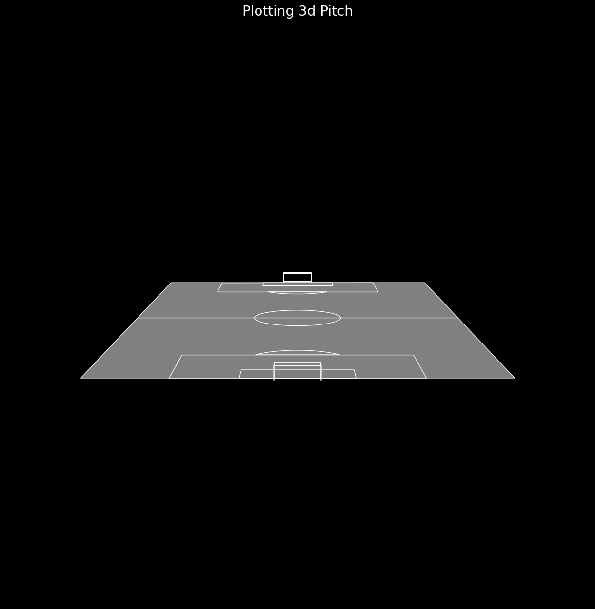
If you set theta = 80 and phi = 40, you will get the following.
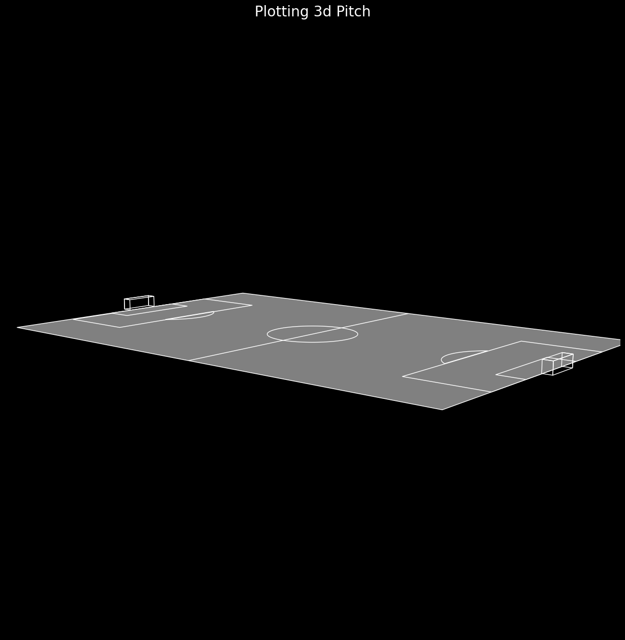
Cool, yeah ?! It definitely looks slick to me. I will leave it as a homework exercise for you to fiddle around with the two axis limit setting lines until you find something that looks good(getting rid of the extra spaces at the top and bottom). Oh, and if you are tired of manually inputting the values, don’t worry - ipywidgets got you covered. Just do the following :
Click to expand!
phi_vals = widgets.FloatSlider(
    value=10,
    min=0,
    max=360.0,
    step=10,
    description="Phi:",
    disabled=False,
    continuous_update=False,
    orientation="horizontal",
    readout=True,
    readout_format=".1f",
)

theta_vals = widgets.FloatSlider(
    value=80,
    min=0,
    max=180.0,
    step=10,
    description="Theta:",
    disabled=False,
    continuous_update=False,
    orientation="horizontal",
    readout=True,
    readout_format=".1f",
)

interactive(viewer, theta=theta_vals, phi=phi_vals)
Now you can drag the sliders and change the orientation of the 3d pitch. My recommendations - keep theta fixed between 60 and 90, and just change phi.
Task 2 : Draw a straight 3d line - a straight shot into the roof of the net.
Here we will need some data. You are free to collect your own data or find from some attainable source. I am going to work with some fake data here. Let’s say we have a penalty, and it is smashed into the top left corner (left from the shooter’s perspective) Ezequiel Garay-style. The start coordinates of the shot are [94,34,0] and the end coordinates are [105,36,2.3] (I am assuming a goal height of 2.4 meters). And it’s hit so hard it just flies straight in (straight line approximation for a small part of the parabola). How do we plot this ?
Well, for the most part, the code remains the same….we plot the pitch as usual like in the first part. Then we add coordinates for the shot itself and plot that. That’s it….that simple once you complete the heavy-lifting in the first part.
Oh, and since it’s a penalty, we don’t need to plot the entire pitch. We could just plot a small area surrounding the penalty box to have a better zoomed-in view. This is a hack, a better way would be to shift the position of the camera but that will require changing a part in the source code, so unless you are prepared to do that, just follow the hack for now.
We will start by re-specifying the vertices and faces of the required lines and also add the shot in.
Click to expand!
pitch_outline = np.array(
    [
        [80.0, 0.0, 0.0],
        [105.0, 0.0, 0.0],
        [105.0, 68.0, 0.0],
        [80.0, 68.0, 0.0],
    ]
)
f_pitch_outline = [[0, 1, 2, 3]]

right_penalty_box = np.array(
    [
        [88.5, 13.84, 0.0],
        [105.0, 13.84, 0.0],
        [105.0, 54.16, 0.0],
        [88.5, 54.16, 0.0],
    ]
)

f_right_penalty_box = [[0, 1, 2, 3]]

right_6yd_box = np.array(
    [
        [99.5, 24.84, 0.0],
        [105.0, 24.84, 0.0],
        [105.0, 43.16, 0.0],
        [99.5, 43.16, 0.0],
    ]
)

f_right_6yd_box = [[0, 1, 2, 3]]

def int_angles(radius, h, k, line_y):
    x1 = h + np.sqrt(radius**2 - (line_y - k) ** 2)
    x2 = h - np.sqrt(radius**2 - (line_y - k) ** 2)
    theta1 = np.arccos((x1 - h) / radius)
    theta2 = np.pi - theta1
    return theta1, theta2

theta1, theta2 = int_angles(9.15, 34, 94, 88.5)
lin1 = np.linspace(np.pi / 2 + theta1, np.pi / 2 + theta2, 200)
right_arc = np.array(
    [94 + 9.15 * np.cos(lin1), 34 + 9.15 * np.sin(lin1), np.zeros(200)]
).transpose()

f_right_arc = [[i for i in range(len(right_arc))]]

right_goal = np.array(
    [
        [105, 30.34, 0.0],
        [105, 30.34, 2.4],
        [105, 37.66, 2.4],
        [105, 37.66, 0],
        [107, 30.34, 0.0],
        [107, 30.34, 2.4],
        [107, 37.66, 2.4],
        [107, 37.66, 0],
    ]
)

f_right_goal = [[4, 5, 6, 7], [0, 1, 5, 4], [2, 6, 7, 3], [1, 2, 6, 5]]

x0, y0, z0, x1, y1, z1 = 94, 34, 0, 105, 36, 2.3

xx = np.linspace(x0, x1, 10)
yy = np.linspace(y0, y1, 10)
zz = np.linspace(z0, z1, 10)

shot = np.array([[xx[i], yy[i], zz[i]] for i in range(10)])
f_shot = [[i for i in range(len(shot))]]
Then we will plot everything, showing the shot in red. We need to make a tiny change in the camera transform function - re-center it and also re-normalize to display in a unit box. The code bits are given below
Click to expand!
def camera_transform(params, vertices, faces, indx, ax, fc, ec):
    vertices[:, 0] = (vertices[:, 0] - 92.5) / 12.5
    vertices[:, 1] = (vertices[:, 1] - 34) / 12.5
    vertices[:, 2] = (vertices[:, 2] - 2.5 / 2) / 12.5
    camera = Camera("perspective", params[0], params[1], scale=0.8)
    vertices = glm.transform(vertices, camera.transform)

    faces = np.array([vertices[face] for face in faces])
    index = np.argsort(-np.mean(faces[..., 2].squeeze(), axis=-1))
    vertices = faces[index][..., :2]

    collection = PolyCollection(vertices, facecolor=fc, edgecolor=ec)
    ax.add_collection(collection)
    return ax


def viewer(theta, phi):
    fig = plt.figure(figsize=(12, 12))
    ax = fig.add_axes([0, 0, 1, 1], xlim=[-1, 1], ylim=[-1, 1], aspect=1)
    ax.axis("off")
    ax.set_title("Plotting 3d Pitch", color="w", fontsize=20)
    fig.set_facecolor("k")
    ax.set_facecolor("k")

    camera_transform(
        params=[theta, phi],
        vertices=pitch_outline.copy(),
        faces=f_pitch_outline.copy(),
        indx=1,
        ax=ax,
        fc="grey",
        ec="w",
    )
    camera_transform(
        params=[theta, phi],
        vertices=right_penalty_box.copy(),
        faces=f_right_penalty_box.copy(),
        indx=1,
        ax=ax,
        fc="grey",
        ec="w",
    )

    camera_transform(
        params=[theta, phi],
        vertices=right_6yd_box.copy(),
        faces=f_right_6yd_box.copy(),
        indx=1,
        ax=ax,
        fc="grey",
        ec="w",
    )

    camera_transform(
        params=[theta, phi],
        vertices=right_arc.copy(),
        faces=f_right_arc.copy(),
        indx=1,
        ax=ax,
        fc="none",
        ec="w",
    )

    camera_transform(
        params=[theta, phi],
        vertices=right_goal.copy(),
        faces=f_right_goal.copy(),
        indx=1,
        ax=ax,
        fc="none",
        ec="w",
    )
    camera_transform(
        params=[theta, phi],
        vertices=shot.copy(),
        faces=f_shot.copy(),
        indx=1,
        ax=ax,
        fc="tab:red",
        ec="tab:red",
    )
    plt.show()
Then choose your favourite angle and display, or use the ipywidgets to rotate things around and marvel at the penalty from a variety of angles. Choosing theta = 60 and phi = 280 produces the following
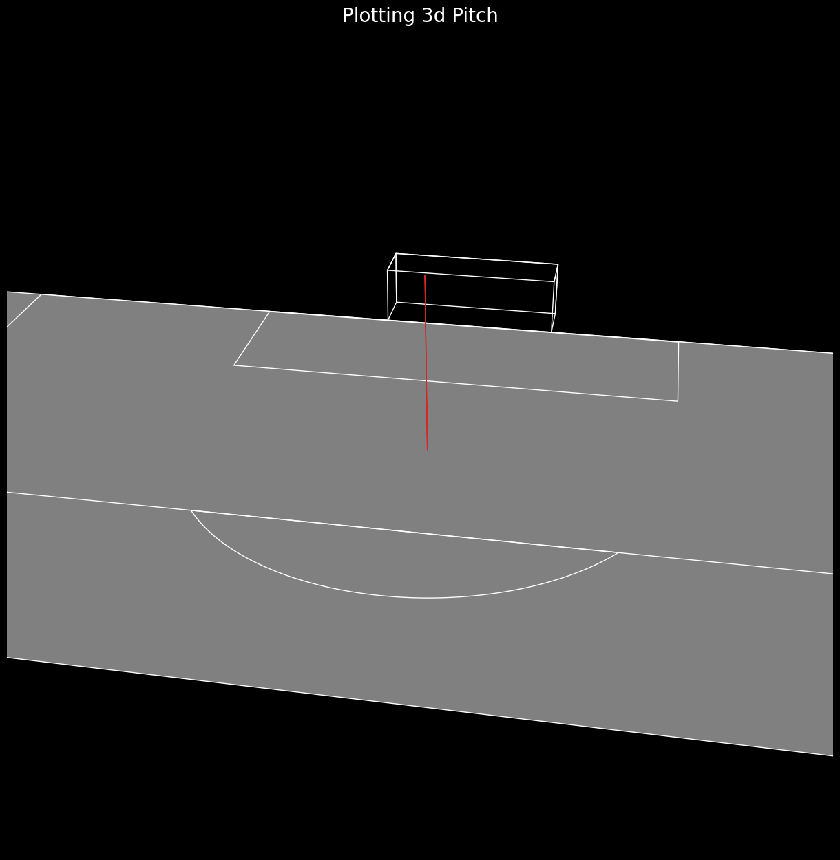
Voila !!
Task 3 : Draw a parabola - say, a long 40 m pass.
To draw a unique straight line you only need to know about two points. To draw unique conic sections (like circles, parabolas, ellipses, hyperbolas) you need three or more. Or, you need to have special information about the points you choose. What do I mean by that ? Suppose the goalkick starts from [5.5, 24.84, 0] - so the right edge of the 6yd box. And it ends at [45, 12, 0] - so a medium-ish kick. If we assume that there is no air resistance, no spin of the ball etc, then the trajectory of the ball is given by a parabola (hence the title of this section). However, we are going to use a special point to draw the parabola….the top-most point/maximum height the ball can reach. Now, this is info you will not get from any free data source. So, you will have to eyeball this info from video footage. Say the ball reached a maximum height of 10 m from the ground. By symmetry, this is also the midpoint of the trajectory, so the coordinates of this point are [25.25, 18.42, 10]. Now we know everything we need to know. We will also assume acceleration due to gravity is 10. Some math is required to work out the trajectory completely - we need the height of the ball at every point. I will show it via the following code snippet
Click to expand!
x0, y0, z0, x1, y1, z1 = 5.5, 24.84, 0, 45, 12, 0
xT,yT,zT = (x1+x0)/2, (y1+y0)/2, 10
xx = np.linspace(x0, x1, 100)
yy = np.linspace(y0, y1, 100)
r = np.sqrt((xx - x0) ** 2 + (yy - y0) ** 2)
R = np.sqrt((xT - x0) ** 2 + (yT - y0) ** 2)
g = 10.0
uz = np.sqrt(2 * g * (zT - z0))
T = uz / g
ur = R / T
zz = uz * r / ur - 0.5 * g * (r / ur) ** 2 + z0

long_pass = np.array([[xx[i], yy[i], zz[i]] for i in range(100)])
long_pass = np.append(long_pass, long_pass[::-1], axis=0)
f_long_pass = [[i for i in range(len(long_pass))]]
Now we go back to using the original full-pitch camera transform function from the first part, add this long pass to the viewer function and plot out in red.
Click to expand!
phi_vals = widgets.FloatSlider(
value=10,
min=0,
max=360.0,
step=10,
description="Phi:",
disabled=False,
continuous_update=False,
orientation="horizontal",
readout=True,
readout_format=".1f",
)
theta_vals = widgets.FloatSlider(
value=80,
min=0,
max=180.0,
step=10,
description="Theta:",
disabled=False,
continuous_update=False,
orientation="horizontal",
readout=True,
readout_format=".1f",
)
def camera_transform(params, vertices, faces, indx, ax, fc, ec):
vertices[:, 0] = (vertices[:, 0] - 52.5) / 52.5
vertices[:, 1] = (vertices[:, 1] - 34) / 52.5
vertices[:, 2] = (vertices[:, 2] - 2.5 / 2) / 52.5
camera = Camera("perspective", params[0], params[1], scale=0.8)
vertices = glm.transform(vertices, camera.transform)
faces = np.array([vertices[face] for face in faces])
index = np.argsort(-np.mean(faces[..., 2].squeeze(), axis=-1))
vertices = faces[index][..., :2]
collection = PolyCollection(vertices, facecolor=fc, edgecolor=ec)
ax.add_collection(collection)
return ax
def viewer(theta, phi):
fig = plt.figure(figsize=(12, 12))
ax = fig.add_axes([0, 0, 1, 1], xlim=[-1, 1], ylim=[-1, 1], aspect=1)
ax.axis("off")
ax.set_title("Plotting 3d Pitch", color="w", fontsize=20)
fig.set_facecolor("k")
ax.set_facecolor("k")
camera_transform(
params=[theta, phi],
vertices=pitch_outline.copy(),
faces=f_pitch_outline.copy(),
indx=1,
ax=ax,
fc="grey",
ec="w",
)
camera_transform(
params=[theta, phi],
vertices=right_penalty_box.copy(),
faces=f_right_penalty_box.copy(),
indx=1,
ax=ax,
fc="grey",
ec="w",
)
camera_transform(
params=[theta, phi],
vertices=left_penalty_box.copy(),
faces=f_left_penalty_box.copy(),
indx=1,
ax=ax,
fc="grey",
ec="w",
)
camera_transform(
params=[theta, phi],
vertices=right_6yd_box.copy(),
faces=f_right_6yd_box.copy(),
indx=1,
ax=ax,
fc="grey",
ec="w",
)
camera_transform(
params=[theta, phi],
vertices=left_6yd_box.copy(),
faces=f_left_6yd_box.copy(),
indx=1,
ax=ax,
fc="grey",
ec="w",
)
camera_transform(
params=[theta, phi],
vertices=centerline.copy(),
faces=f_centerline.copy(),
indx=1,
ax=ax,
fc="grey",
ec="w",
)
camera_transform(
params=[theta, phi],
vertices=centercircle.copy(),
faces=f_centercircle.copy(),
indx=1,
ax=ax,
fc="none",
ec="w",
)
camera_transform(
params=[theta, phi],
vertices=right_arc.copy(),
faces=f_right_arc.copy(),
indx=1,
ax=ax,
fc="none",
ec="w",
)
camera_transform(
params=[theta, phi],
vertices=left_arc.copy(),
faces=f_left_arc.copy(),
indx=1,
ax=ax,
fc="none",
ec="w",
)
camera_transform(
params=[theta, phi],
vertices=right_goal.copy(),
faces=f_right_goal.copy(),
indx=1,
ax=ax,
fc="none",
ec="w",
)
camera_transform(
params=[theta, phi],
vertices=left_goal.copy(),
faces=f_left_goal.copy(),
indx=1,
ax=ax,
fc="none",
ec="w",
)
camera_transform(
params=[theta, phi],
vertices=long_pass.copy(),
faces=f_long_pass.copy(),
indx=1,
ax=ax,
fc="none",
ec="tab:red",
)
plt.show()
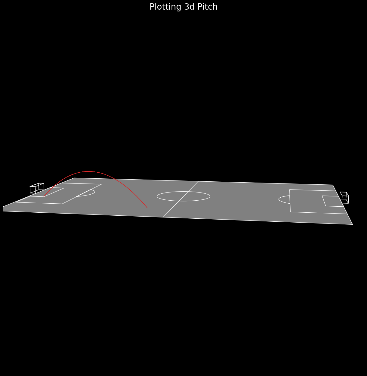
interactive(viewer, theta=theta_vals, phi=phi_vals)Setting the angles to theta = 80, phi = 10 produces the following
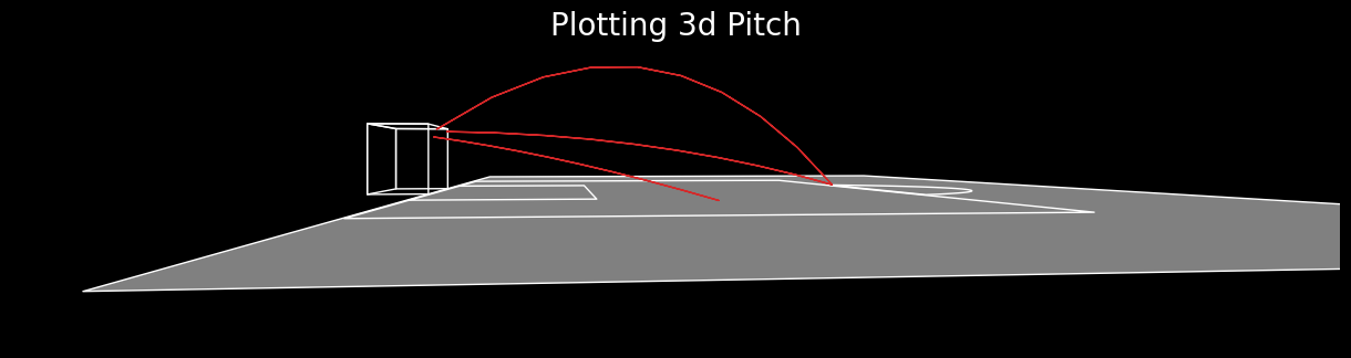
Task 4 : Plot shots with dip
This is the final bit…plotting dipping shots. I will show you three different shots. All parabolic curves. The first one enters the goal when the ball is at its topmost point of the parabolic trajectory. The second one reaches up to the topmost point and then dips down. The third one is from close range and enters the goal without ever hitting the topmost point of the trajectory. The first two cases, you can pretty much handle them the way the long goal kick was handled. For the third case, since we do not know/have a guesstimate of the topmost point, its better to guesstimate the initial angle of the shot. Its typically going to be small (around 10-15 degrees). I will once again show the math details in the code itself…reach out if you have further questions. The inputs you need for each shot are as follows :
Shot 2 : starting point [x0, y0, z0] : [88, 25, 0] ending point [x1, y1, z1] : [105, 31, 2.3] topmost point is the same as the ending point
Shot 2 : starting point [x0, y0, z0] : [88, 25, 0] ending point [x1, y1, z1] : [105, 35, 2.3] maximum height reached zT = 5
Shot 3 : starting point [x0, y0, z0] : [96, 45, 0] ending point [x1, y1, z1] : [105, 36, 2] intial angle theta0 = np.deg2rad(12)
Click to expand!
pitch_outline = np.array(
    [
        [80.0, 0.0, 0.0],
        [105.0, 0.0, 0.0],
        [105.0, 68.0, 0.0],
        [80.0, 68.0, 0.0],
    ]
)
f_pitch_outline = [[0, 1, 2, 3]]

right_penalty_box = np.array(
    [
        [88.5, 13.84, 0.0],
        [105.0, 13.84, 0.0],
        [105.0, 54.16, 0.0],
        [88.5, 54.16, 0.0],
    ]
)

f_right_penalty_box = [[0, 1, 2, 3]]

right_6yd_box = np.array(
    [
        [99.5, 24.84, 0.0],
        [105.0, 24.84, 0.0],
        [105.0, 43.16, 0.0],
        [99.5, 43.16, 0.0],
    ]
)

f_right_6yd_box = [[0, 1, 2, 3]]

def int_angles(radius, h, k, line_y):
    x1 = h + np.sqrt(radius**2 - (line_y - k) ** 2)
    x2 = h - np.sqrt(radius**2 - (line_y - k) ** 2)
    theta1 = np.arccos((x1 - h) / radius)
    theta2 = np.pi - theta1
    return theta1, theta2

theta1, theta2 = int_angles(9.15, 34, 94, 88.5)
lin1 = np.linspace(np.pi / 2 + theta1, np.pi / 2 + theta2, 200)
right_arc = np.array(
    [94 + 9.15 * np.cos(lin1), 34 + 9.15 * np.sin(lin1), np.zeros(200)]
).transpose()

f_right_arc = [[i for i in range(len(right_arc))]]

right_goal = np.array(
    [
        [105, 30.34, 0.0],
        [105, 30.34, 2.4],
        [105, 37.66, 2.4],
        [105, 37.66, 0],
        [107, 30.34, 0.0],
        [107, 30.34, 2.4],
        [107, 37.66, 2.4],
        [107, 37.66, 0],
    ]
)

f_right_goal = [[4, 5, 6, 7], [0, 1, 5, 4], [2, 6, 7, 3], [1, 2, 6, 5]]

#### Shot 1

x0, y0, z0, x1, y1, z1 = 88, 25, 0, 105, 31, 2.3
xT,yT,zT = x1,y1,z1

xx = np.linspace(x0, x1, 10)
yy = np.linspace(y0, y1, 10)
r = np.sqrt((xx - x0) ** 2 + (yy - y0) ** 2)
R = np.sqrt((x1 - x0) ** 2 + (y1 - y0) ** 2)
g = 10.0
uz = np.sqrt(2 * g * (zT - z0))
T = uz / g
ur = R / T
zz = uz * r / ur - 0.5 * g * (r / ur) ** 2 + z0
shot1 = np.array([[xx[i], yy[i], zz[i]] for i in range(10)])
shot1 = np.append(shot1, shot1[::-1], axis=0)
f_shot1 = [[i for i in range(len(shot1))]]


#### Shot 2

x0, y0, z0, x1, y1, z1 = 88, 25, 0, 105, 35, 2.3
zT = 5

xx = np.linspace(x0, x1, 10)
yy = np.linspace(y0, y1, 10)
r = np.sqrt((xx - x0) ** 2 + (yy - y0) ** 2)
g = 10.0
uz = np.sqrt(2 * g * (zT - z0))
T = uz / g

r1 = np.sqrt((x1 - x0) ** 2 + (y1 - y0) ** 2)
a = 0.5*g*T**2
b = -uz*T
c = z1-z0

R = r1*2*a/(-b + np.sqrt(b**2 - 4*a*c))
ur = R/T

zz = uz * r / ur - 0.5 * g * (r / ur) ** 2 + z0
shot2 = np.array([[xx[i], yy[i], zz[i]] for i in range(10)])
shot2 = np.append(shot2, shot2[::-1], axis=0)
f_shot2 = [[i for i in range(len(shot2))]]

#### Shot 3

x0, y0, z0, x1, y1, z1 = 96, 45, 0, 105, 36, 2
theta0 = np.deg2rad(12)

xx = np.linspace(x0, x1, 10)
yy = np.linspace(y0, y1, 10)
r = np.sqrt((xx - x0) ** 2 + (yy - y0) ** 2)
r1  = np.sqrt((x1 - x0) ** 2 + (y1 - y0) ** 2)
g = 10.0
u = np.sqrt(0.5*g*r1**2/(  (r1*np.tan(theta0) - (z1-z0))*(np.cos(theta0))**2) )

zz =r*np.tan(theta0) - 0.5 * g * (r / (u*np.cos(theta0))) ** 2 + z0
shot3 = np.array([[xx[i], yy[i], zz[i]] for i in range(10)])
shot3 = np.append(shot3, shot3[::-1], axis=0)
f_shot3 = [[i for i in range(len(shot3))]]
Note that I am only choosing to plot a part of the pitch to zoom in onto the shots. Now comes the final plotting bit.
Click to expand!
### Plotting pitches

phi_vals = widgets.FloatSlider(
    value=10,
    min=0,
    max=360.0,
    step=10,
    description="Phi:",
    disabled=False,
    continuous_update=False,
    orientation="horizontal",
    readout=True,
    readout_format=".1f",
)

theta_vals = widgets.FloatSlider(
    value=80,
    min=0,
    max=180.0,
    step=10,
    description="Theta:",

    disabled=False,
    continuous_update=False,
    orientation="horizontal",
    readout=True,
    readout_format=".1f",
)


def camera_transform(params, vertices, faces, indx, ax, fc, ec):
    vertices[:, 0] = (vertices[:, 0] - 92.5) / 12.5
    vertices[:, 1] = (vertices[:, 1] - 34) / 12.5
    vertices[:, 2] = (vertices[:, 2] - 2.5 / 2) / 12.5
    camera = Camera("perspective", params[0], params[1], scale=0.8)
    vertices = glm.transform(vertices, camera.transform)

    faces = np.array([vertices[face] for face in faces])
    index = np.argsort(-np.mean(faces[..., 2].squeeze(), axis=-1))
    vertices = faces[index][..., :2]

    collection = PolyCollection(vertices, facecolor=fc, edgecolor=ec)
    ax.add_collection(collection)

    ax.set_ylim(-0.5, 0.3)
    ax.set_xlim(-2, 1.5)
    return ax


def viewer(theta, phi):
    fig = plt.figure(figsize=(12, 12))
    ax = fig.add_axes([0, 0, 1, 1], xlim=[-1, 1], ylim=[-1, 1], aspect=1)
    ax.axis("off")
    ax.set_title("Plotting 3d Pitch", color="w", fontsize=20)
    fig.set_facecolor("k")
    ax.set_facecolor("k")

    camera_transform(
        params=[theta, phi],
        vertices=pitch_outline.copy(),
        faces=f_pitch_outline.copy(),
        indx=1,
        ax=ax,
        fc="grey",
        ec="w",
    )
    camera_transform(
        params=[theta, phi],
        vertices=right_penalty_box.copy(),
        faces=f_right_penalty_box.copy(),
        indx=1,
        ax=ax,
        fc="grey",
        ec="w",
    )

    camera_transform(
        params=[theta, phi],
        vertices=right_6yd_box.copy(),
        faces=f_right_6yd_box.copy(),
        indx=1,
        ax=ax,
        fc="grey",
        ec="w",
    )

    camera_transform(
        params=[theta, phi],
        vertices=right_arc.copy(),
        faces=f_right_arc.copy(),
        indx=1,
        ax=ax,
        fc="none",
        ec="w",
    )

    camera_transform(
        params=[theta, phi],
        vertices=right_goal.copy(),
        faces=f_right_goal.copy(),
        indx=1,
        ax=ax,
        fc="none",
        ec="w",
    )
    camera_transform(
        params=[theta, phi],
        vertices=shot1.copy(),
        faces=f_shot1.copy(),
        indx=1,
        ax=ax,
        fc="tab:red",
        ec="tab:red",
    )
    camera_transform(
        params=[theta, phi],
        vertices=shot2.copy(),
        faces=f_shot2.copy(),
        indx=1,
        ax=ax,
        fc="tab:red",
        ec="tab:red",
    )
    camera_transform(
        params=[theta, phi],
        vertices=shot3.copy(),
        faces=f_shot3.copy(),
        indx=1,
        ax=ax,
        fc="tab:red",
        ec="tab:red",
    )
    plt.show()


interactive(viewer, theta=theta_vals, phi=phi_vals)
Setting the angles to theta = 90, phi = 170 produces the following
Play with the angles, and have fun. This brings an end to this article. There can be a ton of other things done - introducing spin, air drag effects etc - maybe I will revisit some of those in a later article. Brad (@DymondFormation) has done a full thesis of work on that so reach out to him for more details regarding shot modelling.
Finally I will end with a brief rant. I am hiding it so click and read only if you want to hear an old man ranting at the clouds…otherwise, what are you waiting for ? Open a jupyter/google colab notebook and get going…try some of these out !! Happy plotting.